
Protein secondary structure
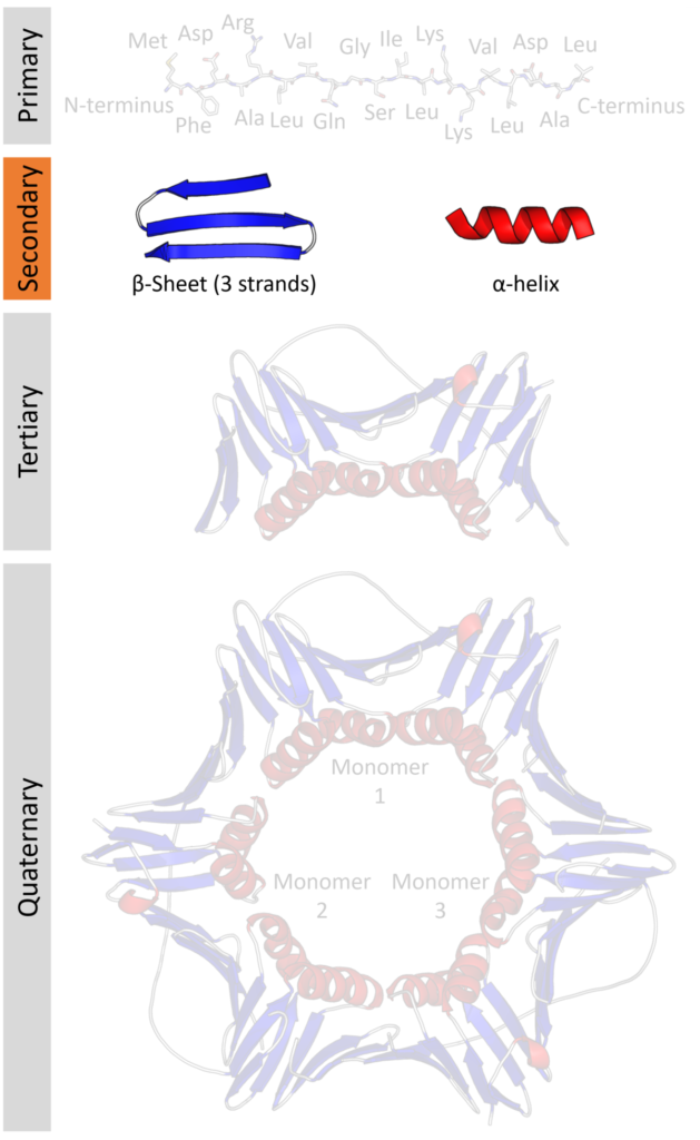
Protein secondary structure is the three dimensional form of local segments of proteins. The two most common secondary structural elements are alpha helices and beta sheets, though beta turns and omega loops occur as well. Secondary structure elements typically spontaneously form as an intermediate before the protein folds into its three dimensional tertiary structure.
Secondary structure is formally defined by the pattern of hydrogen bonds between the amino hydrogen and carboxyl oxygen atoms in the peptide backbone. Secondary structure may alternatively be defined based on the regular pattern of backbone dihedral angles in a particular region of the Ramachandran plot regardless of whether it has the correct hydrogen bonds.
The concept of secondary structure was first introduced by Kaj Ulrik Linderstrøm-Lang at Stanford in 1952.
- Linderstrøm-Lang KU (1952). Lane Medical Lectures: Proteins and Enzymes. Stanford University Press. p. 115. ASIN B0007J31SC.
- Schellman JA, Schellman CG (1997). “Kaj Ulrik Linderstrøm-Lang (1896–1959)”. Protein Sci. 6 (5): 1092–100. doi:10.1002/pro.5560060516. PMC 2143695. PMID 9144781.
He had already introduced the concepts of the primary, secondary, and tertiary structure of proteins in the third Lane Lecture (Linderstram-Lang, 1952)
Other types of biopolymers such as nucleic acids also possess characteristic secondary structures.
Types
| Geometry attribute | α-helix | 310 helix | π-helix |
|---|---|---|---|
| Residues per turn | 3.6 | 3.0 | 4.4 |
| Translation per residue | 1.5 Å (0.15 nm) | 2.0 Å (0.20 nm) | 1.1 Å (0.11 nm) |
| Radius of helix | 2.3 Å (0.23 nm) | 1.9 Å (0.19 nm) | 2.8 Å (0.28 nm) |
| Pitch | 5.4 Å (0.54 nm) | 6.0 Å (0.60 nm) | 4.8 Å (0.48 nm) |
Steven Bottomley (2004). “Interactive Protein Structure Tutorial”. Archived from the original on March 1, 2011. Retrieved January 9, 2011. Schulz, G. E. (Georg E.), 1939- (1979). Principles of protein structure. Schirmer, R. Heiner, 1942-. New York: Springer-Verlag. ISBN 0-387-90386-0. OCLC 4498269. Schulz, G. E. (Georg E.), 1939- (1979). Principles of protein structure. Schirmer, R. Heiner, 1942-. New York: Springer-Verlag. ISBN 0-387-90386-0. OCLC 4498269.
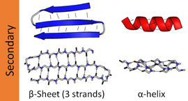
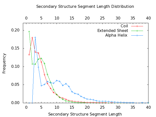
The most common secondary structures are alpha helices and beta sheets. Other helices, such as the 310 helix and π helix, are calculated to have energetically favorable hydrogen-bonding patterns but are rarely observed in natural proteins except at the ends of α helices due to unfavorable backbone packing in the center of the helix. Other extended structures such as the polyproline helix and alpha sheet are rare in native state proteins but are often hypothesized as important protein folding intermediates. Tight turns and loose, flexible loops link the more “regular” secondary structure elements. The random coil is not a true secondary structure, but is the class of conformations that indicate an absence of regular secondary structure.
Amino acids vary in their ability to form the various secondary structure elements. Proline and glycine are sometimes known as “helix breakers” because they disrupt the regularity of the α helical backbone conformation; however, both have unusual conformational abilities and are commonly found in turns. Amino acids that prefer to adopt helical conformations in proteins include methionine, alanine, leucine, glutamate and lysine (“MALEK” in amino-acid 1-letter codes); by contrast, the large aromatic residues (tryptophan, tyrosine and phenylalanine) and Cβ-branched amino acids (isoleucine, valine, and threonine) prefer to adopt β-strand conformations. However, these preferences are not strong enough to produce a reliable method of predicting secondary structure from sequence alone.
Low frequency collective vibrations are thought to be sensitive to local rigidity within proteins, revealing beta structures to be generically more rigid than alpha or disordered proteins.
- Perticaroli S, Nickels JD, Ehlers G, O’Neill H, Zhang Q, Sokolov AP (October 2013). “Secondary structure and rigidity in model proteins”. Soft Matter. 9 (40): 9548–56. Bibcode:2013SMat….9.9548P. doi:10.1039/C3SM50807B. PMID 26029761.
- Perticaroli S, Nickels JD, Ehlers G, Sokolov AP (June 2014). “Rigidity, secondary structure, and the universality of the boson peak in proteins”. Biophysical Journal. 106 (12): 2667–74. Bibcode:2014BpJ…106.2667P. doi:10.1016/j.bpj.2014.05.009. PMC 4070067. PMID 24940784.
Neutron scattering measurements have directly connected the spectral feature at ~1 THz to collective motions of the secondary structure of beta-barrel protein GFP.
- Nickels JD, Perticaroli S, O’Neill H, Zhang Q, Ehlers G, Sokolov AP (2013). “Coherent neutron scattering and collective dynamics in the protein, GFP”. Biophys. J. 105 (9): 2182–87. Bibcode:2013BpJ…105.2182N. doi:10.1016/j.bpj.2013.09.029. PMC 3824694. PMID 24209864.
Hydrogen bonding patterns in secondary structures may be significantly distorted, which makes automatic determination of secondary structure difficult. There are several methods for formally defining protein secondary structure, e.g.,
- DSSP,
- Kabsch W, Sander C (Dec 1983). “Dictionary of protein secondary structure: pattern recognition of hydrogen-bonded and geometrical features”. Biopolymers. 22 (12): 2577–637. doi:10.1002/bip.360221211. PMID 6667333. S2CID 29185760.
- The DSSP algorithm is the standard method for assigning secondary structure to the amino acids of a protein, given the atomic-resolution coordinates of the protein. The abbreviation is only mentioned once in the 1983 paper describing this algorithm,
- where it is the name of the Pascal program that implements the algorithm Define Secondary Structure of Proteins.
- DSSP begins by identifying the intra-backbone hydrogen bonds of the protein using a purely electrostatic definition, assuming partial charges of -0.42 e and +0.20 e to the carbonyl oxygen and amide hydrogen respectively, their opposites assigned to the carbonyl carbon and amide nitrogen. A hydrogen bond is identified if E in the following equation is less than -0.5 kcal/mol:{\displaystyle E=0.084\left\{{\frac {1}{r_{ON}}}+{\frac {1}{r_{CH}}}-{\frac {1}{r_{OH}}}-{\frac {1}{r_{CN}}}\right\}\cdot 332\,\mathrm {kcal/mol} }
where the {\displaystyle r_{AB}}
terms indicate the distance between atoms A and B, taken from the carbon (C) and oxygen (O) atoms of the C=O group and the nitrogen (N) and hydrogen (H) atoms of the N-H group.
- Based on this, eight types of secondary structure are assigned. The 310 helix, α helix and π helix have symbols G, H and I and are recognized by having a repetitive sequence of hydrogen bonds in which the residues are three, four, or five residues apart respectively. Two types of beta sheet structures exist; a beta bridge has symbol B while longer sets of hydrogen bonds and beta bulges have symbol E. T is used for turns, featuring hydrogen bonds typical of helices, S is used for regions of high curvature (where the angle between {\displaystyle {\overrightarrow {C_{i}^{\alpha }C_{i+2}^{\alpha }}}}
and {\displaystyle {\overrightarrow {C_{i-2}^{\alpha }C_{i}^{\alpha }}}}
is at least 70°), and a blank (or space) is used if no other rule applies, referring to loops.
- These eight types are usually grouped into three larger classes: helix (G, H and I), strand (E and B) and loop (S, T, and C, where C sometimes is represented also as blank space).
- π helices – In the original DSSP algorithm, residues were preferentially assigned to α helices, rather than π helices. In 2011, it was shown that DSSP failed to annotate many “cryptic” π helices, which are commonly flanked by α helices.
- Cooley RB, Arp DJ, Karplus PA (2010). “Evolutionary origin of a secondary structure: π-helices as cryptic but widespread insertional variations of α-helices enhancing protein functionality”. J Mol Biol. 404 (2): 232–246. doi:10.1016/j.jmb.2010.09.034. PMC 2981643. PMID 20888342.
- In 2012, DSSP was rewritten so that the assignment of π helices was given preference over α helices, resulting in better detection of π helices.
- Versions of DSSP from 2.1.0 onwards therefore produce slightly different output from older versions.
- Variants – In 2002, a continuous DSSP assignment was developed by introducing multiple hydrogen bond thresholds, where the new assignment was found to correlate with protein motion.
- Andersen CA, Palmer AG, Brunak S, Rost B (2002). “Continuum secondary structure captures protein flexibility”. Structure. 10 (2): 175–184. doi:10.1016/S0969-2126(02)00700-1. PMID 11839303.
- Based on this, eight types of secondary structure are assigned. The 310 helix, α helix and π helix have symbols G, H and I and are recognized by having a repetitive sequence of hydrogen bonds in which the residues are three, four, or five residues apart respectively. Two types of beta sheet structures exist; a beta bridge has symbol B while longer sets of hydrogen bonds and beta bulges have symbol E. T is used for turns, featuring hydrogen bonds typical of helices, S is used for regions of high curvature (where the angle between {\displaystyle {\overrightarrow {C_{i}^{\alpha }C_{i+2}^{\alpha }}}}
- Kabsch W, Sander C (Dec 1983). “Dictionary of protein secondary structure: pattern recognition of hydrogen-bonded and geometrical features”. Biopolymers. 22 (12): 2577–637. doi:10.1002/bip.360221211. PMID 6667333. S2CID 29185760.
- DEFINE,
- STRIDE,
- Frishman D, Argos P (Dec 1995). “Knowledge-based protein secondary structure assignment” (PDF). Proteins. 23 (4): 566–79. CiteSeerX 10.1.1.132.9420. doi:10.1002/prot.340230412. PMID 8749853. S2CID 17487756. Archived from the original (PDF) on 2010-06-13.
- In protein structure, STRIDE (Structural identification) is an algorithm for the assignment of protein secondary structure elements given the atomic coordinates of the protein, as defined by X-ray crystallography, protein NMR, or another protein structure determination method. In addition to the hydrogen bond criteria used by the more common DSSP algorithm, the STRIDE assignment criteria also include dihedral angle potentials. As such, its criteria for defining individual secondary structures are more complex than those of DSSP. The STRIDE energy function contains a hydrogen-bond term containing a Lennard-Jones-like 8-6 distance-dependent potential and two angular dependence factors reflecting the planarity of the optimized hydrogen bond geometry. The criteria for individual secondary structural elements, which are divided into the same groups as those reported by DSSP, also contain statistical probability factors derived from empirical examinations of solved structures with visually assigned secondary structure elements extracted from the Protein Data Bank.
- Although DSSP is the older method and continues to be the most commonly used, the original STRIDE definition reported it to give a more satisfactory structural assignment in at least 70% of cases. In particular, STRIDE was observed to correct for the propensity of DSSP to assign shorter secondary structures than would be assigned by an expert crystallographer, usually due to the minor local variations in structure that are most common near the termini of secondary structure elements.
- Frishman D, Argos P. (1995). Knowledge-based protein secondary structure assignment. Proteins 23(4):566-79. doi:10.1002/prot.340230412 PMID 8749853
- Using a sliding-window method to smooth variations in assignment of single terminal residues, current implementations of STRIDE and DSSP are reported to agree in up to 95.4% of cases.
- Both STRIDE and DSSP, among other common secondary structure assignment methods, are believed to underpredict pi helices.
- Frishman D, Argos P (Dec 1995). “Knowledge-based protein secondary structure assignment” (PDF). Proteins. 23 (4): 566–79. CiteSeerX 10.1.1.132.9420. doi:10.1002/prot.340230412. PMID 8749853. S2CID 17487756. Archived from the original (PDF) on 2010-06-13.
- ScrewFit,
- Calligari PA, Kneller GR (December 2012). “ScrewFit: combining localization and description of protein secondary structure”. Acta Crystallographica Section D. 68 (Pt 12): 1690–3. doi:10.1107/s0907444912039029. PMID 23151634.
- SST
- Konagurthu AS, Lesk AM, Allison L (Jun 2012). “Minimum message length inference of secondary structure from protein coordinate data”. Bioinformatics. 28 (12): i97–i105. doi:10.1093/bioinformatics/bts223. PMC 3371855. PMID 22689785.
DSSP classification
Main article: DSSP (protein)
The Dictionary of Protein Secondary Structure, in short DSSP, is commonly used to describe the protein secondary structure with single letter codes. The secondary structure is assigned based on hydrogen bonding patterns as those initially proposed by Pauling et al. in 1951 (before any protein structure had ever been experimentally determined). There are eight types of secondary structure that DSSP defines:
- G = 3-turn helix (310 helix). Min length 3 residues.
- H = 4-turn helix (α helix). Minimum length 4 residues.
- I = 5-turn helix (π helix). Minimum length 5 residues.
- T = hydrogen bonded turn (3, 4 or 5 turn)
- E = extended strand in parallel and/or anti-parallel β-sheet conformation. Min length 2 residues.
- B = residue in isolated β-bridge (single pair β-sheet hydrogen bond formation)
- S = bend (the only non-hydrogen-bond based assignment).
- C = coil (residues which are not in any of the above conformations).
‘Coil’ is often codified as ‘ ‘ (space), C (coil) or ‘–’ (dash). The helices (G, H and I) and sheet conformations are all required to have a reasonable length. This means that 2 adjacent residues in the primary structure must form the same hydrogen bonding pattern. If the helix or sheet hydrogen bonding pattern is too short they are designated as T or B, respectively. Other protein secondary structure assignment categories exist (sharp turns, Omega loops, etc.), but they are less frequently used.
Secondary structure is defined by hydrogen bonding, so the exact definition of a hydrogen bond is critical. The standard hydrogen-bond definition for secondary structure is that of DSSP, which is a purely electrostatic model. It assigns charges of ±q1 ≈ 0.42e to the carbonyl carbon and oxygen, respectively, and charges of ±q2 ≈ 0.20e to the amide hydrogen and nitrogen, respectively. The electrostatic energy is{\displaystyle E=q_{1}q_{2}\left({\frac {1}{r_{\mathrm {ON} }}}+{\frac {1}{r_{\mathrm {CH} }}}-{\frac {1}{r_{\mathrm {OH} }}}-{\frac {1}{r_{\mathrm {CN} }}}\right)\cdot 332{\text{ kcal/mol}}.}

According to DSSP, a hydrogen-bond exists if and only if E is less than −0.5 kcal/mol (−2.1 kJ/mol). Although the DSSP formula is a relatively crude approximation of the physical hydrogen-bond energy, it is generally accepted as a tool for defining secondary structure.
SST classification
- Konagurthu AS, Lesk AM, Allison L (Jun 2012). “Minimum message length inference of secondary structure from protein coordinate data”. Bioinformatics. 28 (12): i97–i105. doi:10.1093/bioinformatics/bts223. PMC 3371855. PMID 22689785.
SST is a Bayesian method to assign secondary structure to protein coordinate data using the Shannon information criterion of Minimum Message Length (MML) inference.
- Minimum message length (MML) is a Bayesian information-theoretic method for statistical model comparison and selection.
- Wallace, C. S. (Christopher S.), -2004. (2005). Statistical and inductive inference by minimum message length. New York: Springer. ISBN 9780387237954. OCLC 62889003.
- It provides a formal information theory restatement of Occam’s Razor: even when models are equal in their measure of fit-accuracy to the observed data, the one generating the most concise explanation of data is more likely to be correct (where the explanation consists of the statement of the model, followed by the lossless encoding of the data using the stated model). MML was invented by Chris Wallace, first appearing in the seminal paper “An information measure for classification”.
- Wallace, C. S.; Boulton, D. M. (1968-08-01). “An Information Measure for Classification”. The Computer Journal. 11 (2): 185–194. doi:10.1093/comjnl/11.2.185. ISSN 0010-4620.
- MML is intended not just as a theoretical construct, but as a technique that may be deployed in practice.
- Allison, Lloyd. (2019). Coding Ockham’s Razor. Springer. ISBN 978-3030094881. OCLC 1083131091.
- It differs from the related concept of Kolmogorov complexity in that it does not require use of a Turing-complete language to model data.
- Wallace, C. S.; Dowe, D. L. (1999-01-01). “Minimum Message Length and Kolmogorov Complexity”. The Computer Journal. 42 (4): 270–283. doi:10.1093/comjnl/42.4.270. ISSN 0010-4620.
SST treats any assignment of secondary structure as a potential hypothesis that attempts to explain (compress) given protein coordinate data. The core idea is that the best secondary structural assignment is the one that can explain (compress) the coordinates of a given protein coordinates in the most economical way, thus linking the inference of secondary structure to lossless data compression. SST accurately delineates any protein chain into regions associated with the following assignment types:
- “SST web server”. Retrieved 17 April 2018.
- E = (Extended) strand of a β-pleated sheet
- G = Right-handed 310 helix
- H = Right-handed α-helix
- I = Right-handed π–helix
- g = Left-handed 310 helix
- h = Left-handed α-helix
- i = Left-handed π–helix
- 3 = 310-like Turn
- 4 = α-like Turn
- 5 = π-like Turn
- T = Unspecified Turn
- C = Coil
- – = Unassigned residue
SST detects π and 310 helical caps to standard α-helices, and automatically assembles the various extended strands into consistent β-pleated sheets. It provides a readable output of dissected secondary structural elements, and a corresponding PyMol-loadable script to visualize the assigned secondary structural elements individually.
Experimental determination
The rough secondary-structure content of a biopolymer (e.g., “this protein is 40% α-helix and 20% β-sheet.”) can be estimated spectroscopically.
- Pelton JT, McLean LR (2000). “Spectroscopic methods for analysis of protein secondary structure”. Anal. Biochem. 277 (2): 167–76. doi:10.1006/abio.1999.4320. PMID 10625503.
For proteins, a common method is far-ultraviolet (far-UV, 170–250 nm) circular dichroism. A pronounced double minimum at 208 and 222 nm indicate α-helical structure, whereas a single minimum at 204 nm or 217 nm reflects random-coil or β-sheet structure, respectively. A less common method is infrared spectroscopy, which detects differences in the bond oscillations of amide groups due to hydrogen-bonding. Finally, secondary-structure contents may be estimated accurately using the chemical shifts of an initially unassigned NMR spectrum.
- Meiler J, Baker D (2003). “Rapid protein fold determination using unassigned NMR data”. Proc. Natl. Acad. Sci. U.S.A. 100 (26): 15404–09. Bibcode:2003PNAS..10015404M. doi:10.1073/pnas.2434121100. PMC 307580. PMID 14668443.
Prediction
See also: Protein structure prediction and List of protein secondary structure prediction programs
Predicting protein tertiary structure from only its amino sequence is a very challenging problem (see protein structure prediction), but using the simpler secondary structure definitions is more tractable.
Early methods of secondary-structure prediction were restricted to predicting the three predominate states: helix, sheet, or random coil. These methods were based on the helix- or sheet-forming propensities of individual amino acids, sometimes coupled with rules for estimating the free energy of forming secondary structure elements. The first widely used techniques to predict protein secondary structure from the amino acid sequence were the Chou–Fasman method
- Chou PY, Fasman GD (Jan 1974). “Prediction of protein conformation”. Biochemistry. 13 (2): 222–45. doi:10.1021/bi00699a002. PMID 4358940.
- Chou PY, Fasman GD (1978). “Empirical predictions of protein conformation”. Annual Review of Biochemistry. 47: 251–76. doi:10.1146/annurev.bi.47.070178.001343. PMID 354496.
- Chou PY, Fasman GD (1978). “Prediction of the secondary structure of proteins from their amino acid sequence”. Advances in Enzymology and Related Areas of Molecular Biology. Advances in Enzymology – and Related Areas of Molecular Biology. Vol. 47. pp. 45–148. doi:10.1002/9780470122921.ch2. ISBN 9780470122921. PMID 364941.
- The Chou–Fasman method is an empirical technique for the prediction of secondary structures in proteins, originally developed in the 1970s by Peter Y. Chou and Gerald D. Fasman. The method is based on analyses of the relative frequencies of each amino acid in alpha helices, beta sheets, and turns based on known protein structures solved with X-ray crystallography. From these frequencies a set of probability parameters were derived for the appearance of each amino acid in each secondary structure type, and these parameters are used to predict the probability that a given sequence of amino acids would form a helix, a beta strand, or a turn in a protein. The method is at most about 50–60% accurate in identifying correct secondary structures,
- which is significantly less accurate than the modern machine learning–based techniques.
- Mount DM (2004). Bioinformatics: Sequence and Genome Analysis (2nd ed.). Cold Spring Harbor, NY: Cold Spring Harbor Laboratory Press. ISBN 978-0-87969-712-9.
and the GOR method.
- Garnier J, Osguthorpe DJ, Robson B (March 1978). “Analysis of the accuracy and implications of simple methods for predicting the secondary structure of globular proteins”. Journal of Molecular Biology. 120 (1): 97–120. doi:10.1016/0022-2836(78)90297-8. PMID 642007.
- The GOR method (short for Garnier–Osguthorpe–Robson) is an information theory-based method for the prediction of secondary structures in proteins. It was developed in the late 1970s shortly after the simpler Chou–Fasman method. Like Chou–Fasman, the GOR method is based on probability parameters derived from empirical studies of known protein tertiary structures solved by X-ray crystallography. However, unlike Chou–Fasman, the GOR method takes into account not only the propensities of individual amino acids to form particular secondary structures, but also the conditional probability of the amino acid to form a secondary structure given that its immediate neighbors have already formed that structure. The method is therefore essentially Bayesian in its analysis.
- Garnier, J.; Gibrat, J. F.; Robson, B. (1996). “GOR method for predicting protein secondary structure from amino acid sequence”. Methods Enzymol. 266: 540–53. doi:10.1016/S0076-6879(96)66034-0. PMID 8743705.
- METHOD: The GOR method analyzes sequences to predict alpha helix, beta sheet, turn, or random coil secondary structure at each position based on 17-amino-acid sequence windows. The original description of the method included four scoring matrices of size 17×20, where the columns correspond to the log-odds score, which reflects the probability of finding a given amino acid at each position in the 17-residue sequence. The four matrices reflect the probabilities of the central, ninth amino acid being in a helical, sheet, turn, or coil conformation. In subsequent revisions to the method, the turn matrix was eliminated due to the high variability of sequences in turn regions (particularly over such a large window). The method was considered as best requiring at least four contiguous residues to score as alpha helices to classify the region as helical, and at least two contiguous residues for a beta sheet.
- Mount, D. M. (2004). Bioinformatics: Sequence and Genome Analysis. Vol. 2. Cold Spring Harbor Laboratory Press. ISBN 0-87969-712-1.
- ALGORITHM: The mathematics and algorithm of the GOR method were based on an earlier series of studies by Robson and colleagues reported mainly in the Journal of Molecular Biology and The Biochemical Journal.
- Robson, B.; Pain, R. H. (1971). “Analysis of the Code Relating Sequence to Conformation in Globular Proteins: Possible Implications for the Mechanism of Formation of Helical Regions”. J. Mol. Biol. 58 (1): 237–256. doi:10.1016/0022-2836(78)90297-8. PMID 642007.
- Robson, B. (1974). “Analysis of the Code Relating Sequence to Conformation in Globular Proteins: Theory and Application of Expected Information”. The Biochemical Journal. 141 (3): 853–867. doi:10.1042/bj1410853. PMC 1168191. PMID 4463965.
- The latter describes the information theoretic expansions in terms of conditional information measures. The use of the word “simple” in the title of the GOR paper reflected the fact that the above earlier methods provided proofs and techniques somewhat daunting by being rather unfamiliar in protein science in the early 1970s; even Bayes methods were then unfamiliar and controversial. An important feature of these early studies, which survived in the GOR method, was the treatment of the sparse protein sequence data of the early 1970s by expected information measures. That is, expectations on a Bayesian basis considering the distribution of plausible information measure values given the actual frequencies (numbers of observations).
- The GOR method (short for Garnier–Osguthorpe–Robson) is an information theory-based method for the prediction of secondary structures in proteins. It was developed in the late 1970s shortly after the simpler Chou–Fasman method. Like Chou–Fasman, the GOR method is based on probability parameters derived from empirical studies of known protein tertiary structures solved by X-ray crystallography. However, unlike Chou–Fasman, the GOR method takes into account not only the propensities of individual amino acids to form particular secondary structures, but also the conditional probability of the amino acid to form a secondary structure given that its immediate neighbors have already formed that structure. The method is therefore essentially Bayesian in its analysis.
Although such methods claimed to achieve ~60% accurate in predicting which of the three states (helix/sheet/coil) a residue adopts, blind computing assessments later showed that the actual accuracy was much lower.
- Kabsch W, Sander C (May 1983). “How good are predictions of protein secondary structure?”. FEBS Letters. 155 (2): 179–82. doi:10.1016/0014-5793(82)80597-8. PMID 6852232. S2CID 41477827.
A significant increase in accuracy (to nearly ~80%) was made by exploiting multiple sequence alignment; knowing the full distribution of amino acids that occur at a position (and in its vicinity, typically ~7 residues on either side) throughout evolution provides a much better picture of the structural tendencies near that position.
- Simossis VA, Heringa J (Aug 2004). “Integrating protein secondary structure prediction and multiple sequence alignment”. Current Protein & Peptide Science. 5 (4): 249–66. doi:10.2174/1389203043379675. PMID 15320732.
- Pirovano W, Heringa J (2010). “Protein secondary structure prediction”. Data Mining Techniques for the Life Sciences. Methods in Molecular Biology. Vol. 609. pp. 327–48. doi:10.1007/978-1-60327-241-4_19. ISBN 978-1-60327-240-7. PMID 20221928.
For illustration, a given protein might have a glycine at a given position, which by itself might suggest a random coil there. However, multiple sequence alignment might reveal that helix-favoring amino acids occur at that position (and nearby positions) in 95% of homologous proteins spanning nearly a billion years of evolution. Moreover, by examining the average hydrophobicity at that and nearby positions, the same alignment might also suggest a pattern of residue solvent accessibility consistent with an α-helix. Taken together, these factors would suggest that the glycine of the original protein adopts α-helical structure, rather than random coil. Several types of methods are used to combine all the available data to form a 3-state prediction, including neural networks, hidden Markov models and support vector machines. Modern prediction methods also provide a confidence score for their predictions at every position.
Secondary-structure prediction methods were evaluated by the Critical Assessment of protein Structure Prediction (CASP) experiments and continuously benchmarked, e.g. by EVA (benchmark). Based on these tests, the most accurate methods were
- Psipred,
- PSI-blast based secondary structure PREDiction (PSIPRED) is a method used to investigate protein structure. It uses artificial neural network machine learning methods in its algorithm.
- Gajendra P. S. Raghava; Harpreet Kaur. “Prediction of beta turn types”. Retrieved 5 May 2014.
- Yi-Ping Phoebe Chen (18 January 2005). Bioinformatics Technologies. Springer. p. 107. ISBN 978-3-540-20873-0.
- Cuff, James A.; Barton, Geoffrey A. (15 August 2000). “Application of multiple sequence alignment profiles to improve protein secondary structure prediction”. Proteins. 40 (3): 502–11. doi:10.1002/1097-0134(20000815)40:3<502::aid-prot170>3.0.co;2-q. PMID 10861942.
- It is a server-side program, featuring a website serving as a front-end interface, which can predict a protein’s secondary structure (beta sheets, alpha helixes and coils) from the primary sequence.
- PSIPRED is available as a web service and as software. The software is distributed as source code, licensed technically as proprietary software. It allows modifying, but enforces freeware provisions by forbidding for-profit distribution of the software and its results.
- PSI-blast based secondary structure PREDiction (PSIPRED) is a method used to investigate protein structure. It uses artificial neural network machine learning methods in its algorithm.
- SAM,
- Karplus K (2009). “SAM-T08, HMM-based protein structure prediction”. Nucleic Acids Res. 37 (Web Server issue): W492–97. doi:10.1093/nar/gkp403. PMC 2703928. PMID 19483096.
- PORTER,
- Pollastri G, McLysaght A (2005). “Porter: a new, accurate server for protein secondary structure prediction”. Bioinformatics. 21 (8): 1719–20. doi:10.1093/bioinformatics/bti203. PMID 15585524.
- PROF,
- Yachdav G, Kloppmann E, Kajan L, Hecht M, Goldberg T, Hamp T, Hönigschmid P, Schafferhans A, Roos M, Bernhofer M, Richter L, Ashkenazy H, Punta M, Schlessinger A, Bromberg Y, Schneider R, Vriend G, Sander C, Ben-Tal N, Rost B (2014). “PredictProtein—an open resource for online prediction of protein structural and functional features”. Nucleic Acids Res. 42 (Web Server issue): W337–43. doi:10.1093/nar/gku366. PMC 4086098. PMID 24799431. and
- SABLE.
The chief area for improvement appears to be the prediction of β-strands; residues confidently predicted as β-strand are likely to be so, but the methods are apt to overlook some β-strand segments (false negatives). There is likely an upper limit of ~90% prediction accuracy overall, due to the idiosyncrasies of the standard method (DSSP) for assigning secondary-structure classes (helix/strand/coil) to PDB structures, against which the predictions are benchmarked.
- Kihara D (Aug 2005). “The effect of long-range interactions on the secondary structure formation of proteins”. Protein Science. 14 (8): 1955–963. doi:10.1110/ps.051479505. PMC 2279307. PMID 15987894.
Accurate secondary-structure prediction is a key element in the prediction of tertiary structure, in all but the simplest (homology modeling) cases. For example, a confidently predicted pattern of six secondary structure elements βαββαβ is the signature of a ferredoxin fold.
- Qi Y, Grishin NV (2005). “Structural classification of thioredoxin-like fold proteins” (PDF). Proteins. 58 (2): 376–88. CiteSeerX 10.1.1.644.8150. doi:10.1002/prot.20329. PMID 15558583. S2CID 823339.
Since the fold definition should include only the core secondary structural elements that are present in the majority of homologs, we define the thioredoxin-like fold as a two-layer α/β sandwich with the βαβββα secondary-structure pattern.
Applications
Both protein and nucleic acid secondary structures can be used to aid in multiple sequence alignment. These alignments can be made more accurate by the inclusion of secondary structure information in addition to simple sequence information. This is sometimes less useful in RNA because base pairing is much more highly conserved than sequence. Distant relationships between proteins whose primary structures are unalignable can sometimes be found by secondary structure.
- Simossis VA, Heringa J (Aug 2004). “Integrating protein secondary structure prediction and multiple sequence alignment”. Current Protein & Peptide Science. 5 (4): 249–66. doi:10.2174/1389203043379675. PMID 15320732.
It has been shown that α-helices are more stable, robust to mutations and designable than β-strands in natural proteins,
- Abrusan G, Marsh JA (2016). “Alpha helices are more robust to mutations than beta strands”. PLOS Computational Biology. 12 (12): e1005242. Bibcode:2016PLSCB..12E5242A. doi:10.1371/journal.pcbi.1005242. PMC 5147804. PMID 27935949.
thus designing functional all-α proteins is likely to be easier that designing proteins with both helices and strands; this has been recently confirmed experimentally.
- Rocklin GJ, et al. (2017). “Global analysis of protein folding using massively parallel design, synthesis, and testing”. Science. 357 (6347): 168–175. Bibcode:2017Sci…357..168R. doi:10.1126/science.aan0693. PMC 5568797. PMID 28706065.
See also
- Folding (chemistry)
- Nucleic acid secondary structure
- Translation
- Structural motif
- Protein circular dichroism data bank
- WHAT IF software
- List of protein secondary structure prediction programs
Further reading
- Branden C, Author J (1999). Introduction to protein structure (2nd ed.). New York: Garland Science. ISBN 978-0815323051.
{{cite book}}:|author=has generic name (help) - Pauling L, Corey RB (1951). “Configurations of Polypeptide Chains With Favored Orientations Around Single Bonds: Two New Pleated Sheets”. Proc. Natl. Acad. Sci. U.S.A. 37 (11): 729–40. Bibcode:1951PNAS…37..729P. doi:10.1073/pnas.37.11.729. PMC 1063460. PMID 16578412. (The original beta-sheet conformation article.)
- Pauling L, Corey RB, Branson HR (1951). “The structure of proteins; two hydrogen-bonded helical configurations of the polypeptide chain”. Proc. Natl. Acad. Sci. U.S.A. 37 (4): 205–11. Bibcode:1951PNAS…37..205P. doi:10.1073/pnas.37.4.205. PMC 1063337. PMID 14816373. (alpha- and pi-helix conformations, since they predicted that {\displaystyle 3_{10}}
helices would not be possible.)
External links
- NetSurfP – Secondary Structure and Surface Accessibility predictor
- PROF
- ScrewFit
- PSSpred A multiple neural network training program for protein secondary structure prediction
- Genesilico metaserver Metaserver which allows to run over 20 different secondary structure predictors by one click
- SST webserver: An information-theoretic (compression-based) secondary structural assignment.
| Protein secondary structure |
|---|
From Wikipedia where the main page was last updated 20 August 2022
Leave a Reply